Variable Local Density Infill

Varying the local density of lattice infill for 3d printing is not a new concept, but the most robust methods typically vary the wall thickness of a fixed cell lattice to achieve a desired density distribution. This works great in technology like SLS/SLA but not so well in FFF, where a specific criteria of infill is that it should be a efficient to print. Most FFF infill patterns are continuous paths with cell walls made of a single extrusion width for this reason (though double/multi-width exists). This makes creating arbitrarily thick walls over a wide domain difficult. This brought me to the idea of varying the size of cells themself to achieve the desired density distribution.

TMPS Infills

My immediate attempts centered around TPMS infill patterns, where you could change the local density by modulating the frequency. Below is a simple one dimensional (frequency modulated over one dimension) version of this, where the frequency of $sin(x)$ at every $x$ is proportional to $0.5x$.

In practice in order to vary the frequency in 3 dimensions you first have to encode your desired density field into a signal function, and then use that to modulate the frequency of the TMPS lattice. The relative density field $\rho$ is turned into instantaneous frequencies $\omega(x, y, z)$ and then encoded into the signal field $\hat{s}$.

Then a phase function is found in all 3 axes, which also applies a smoothing radius $R$.

Then TPMS functions can be evaluated, in this case the gyroid function where.

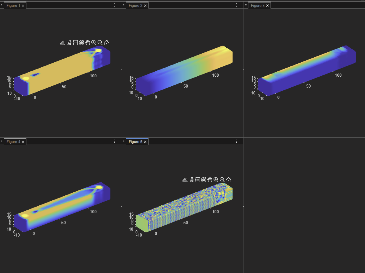Relative density field, $x$, $y$, and $z$ phase function values, and the final gyroid field

Implementation

A framework to test my methods was created in MATLAB, focusing on generating the surfaces rather than creating printable g-code. This is where phase accumulation appeared, creating unprintable artifacts that did not match the target density distribution near any sharp changes in relative density. I had pre-empted this problem with the smoothing radius $R$ as mentioned above but it was insufficient in steep transitions. There were also artifacts outside the part bounds but there were expected and wouldn’t impact final printability.

Smooth Transitions

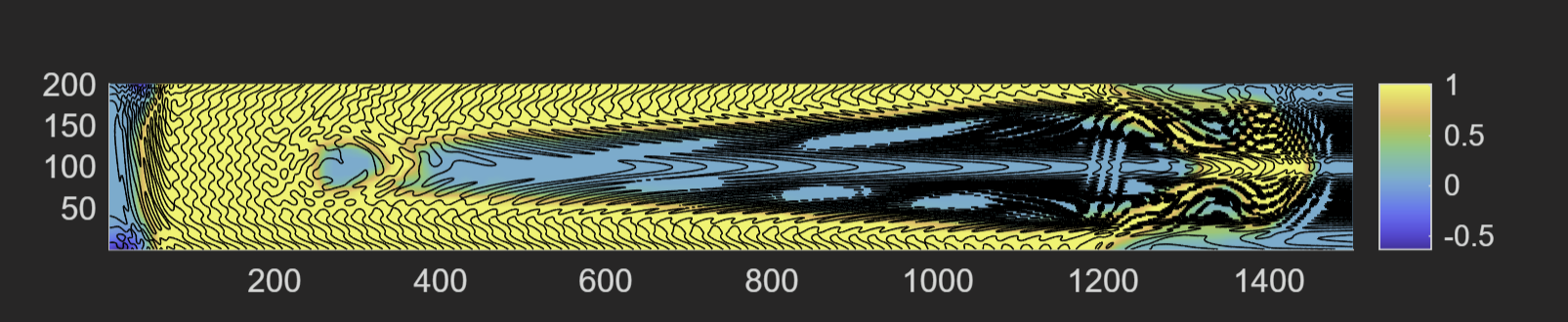Phase Artifacts

Another hurdle in the implementation was computation, writing simple MATLAB code was incredibly inefficient. The first fix was offloading the large matrix operations to the GPU, and the second was performing the integration of the smoothing area via convolution, again on the GPU.

% Calculate phases on meshgrid
% Performs integration with convolution

kernelWidth = round(2 * smoothingRadius / finmeshResolution);
finmeshVoxelArea = finmeshResolution^2;
xKernel = ones(1, kernelWidth, kernelWidth, 'gpuArray') .* finmeshVoxelArea;
yKernel = ones(kernelWidth, 1, kernelWidth, 'gpuArray') .* finmeshVoxelArea;
zKernel = ones(kernelWidth, kernelWidth, 1, 'gpuArray') .* finmeshVoxelArea;

xIntegral = convn(finmesh, xKernel, 'same');
yIntegral = convn(finmesh, yKernel, 'same');
zIntegral = convn(finmesh, zKernel, 'same');
smoothingArea = 4 * smoothingRadius^2;
integralFactor = (omegaDelta / smoothingArea);

xPhase = carrierFrequency .* finmeshXImplicitVector + integralFactor .* cumtrapz(finmeshXVector, xIntegral, 1);
yPhase = carrierFrequency .* finmeshYImplicitVector + integralFactor .* cumtrapz(finmeshYVector, yIntegral, 2);
zPhase = carrierFrequency .* finmeshZImplicitVector + integralFactor .* cumtrapz(finmeshZVector, zIntegral, 3);

inPartX = minX <= finmeshXVector & maxX >= finmeshXVector;
inPartY = minY <= finmeshYVector & maxY >= finmeshYVector;
inPartZ = minZ <= finmeshZVector & maxZ >= finmeshZVector;

xPhase = xPhase(inPartX, inPartY, inPartZ);
yPhase = yPhase(inPartX, inPartY, inPartZ);
zPhase = zPhase(inPartX, inPartY, inPartZ);

finmesh = finmesh(inPartX, inPartY, inPartZ);

Next Steps

It was around getting to this point that I found a paper by Isaac Wegner that outlined a similar (though much more polished) methodology. I reached out to talk about the this method and ended up reimplementing the methods in his paper to confirm my artifacts were not due to an error. This left me with a few paths.

1. Bounding the field & density gradient
   • This would include pre-processing the relative density field to minimize the maximum gradient to a determined acceptable amount, and potentially instituting a lower and upper bound to the relative density values. This avoids instances of high density gradient all together
   • The cons are that it isn’t quite as “native” as generating the field directly, but in practice it is likely to be necessary regardless of the phase accumulation issue as TMPS infills cannot properly approach 100% density in FFF even if uniform, so edge cases would always exist
2. Zoned infill
   • This would likely work with option 1, deliberately selecting “zones” of constant or similar density. This would allow solid structure to exist within the part where needed, and shifts the problem to creating an interface between zones.
3. Recursive cubic (octree)
   • Adaptive cubic infill is an existing infill type where near the edges of parts octree’s are subdivided more. This works as broadly speaking much of the stress is concentrated around the edge of parts in many common cases.
   • Recursive cubic would build on this by changing the subdivision rule. Subdivisions would be created based on a rule such as the ratio of accumulated local density within the division to the volume of the division
   • Cubic infill is more susceptible sudden failure due to imperfection in a single cell or member than a TPMS lattice
   • The closest prior work found for this is the existing adaptive cubic infill.

Recursive Cubic

Initial prototypes of recursive cubic infill on a modified Orca slicer build.